RBF函数插值
径向基函数(Radial Basis Function, RBF)插值的基本形式为
$$
F(\boldsymbol{r})=\sum_{i=1}^N w_i \varphi\left(\left|\boldsymbol{r}-\boldsymbol{r}_i\right|\right)
$$
式中, $F(\boldsymbol{r})$ 是插值函数, $N$ 为插值问题所使用的径向基函数总数目(控制点总数目), $\varphi\left(\left|\boldsymbol{r}-\boldsymbol{r}_i\right|\right)$ 是采用的径向基函数的通用形式, $\left|\boldsymbol{r}-\boldsymbol{r}_i\right|$ 是两个位置矢量的欧氏距离, $\boldsymbol{r}_i$ 是第 $i$ 号径向基函数的控制点位置, $w_i$ 是第 $i$ 号径向基函数对应的权重系数。
径向基函数类型很多,总结有如下六种:
- Gaussian(高斯曲面函数):$\quad \varphi(x)=\exp \left(-\frac{x^2}{2 \sigma^2}\right)$
- Multiquadrics(多项式函数):$\quad \varphi(x)=\sqrt{1+\frac{x^2}{\sigma^2}}$
- Linear(线性函数):$\varphi(x)=x$
- Cubic(立方体曲面函数):$\varphi(x)=x^3$
- Thinplate(薄板曲面函数):$\quad \varphi(x)=x^2 \ln (x+1)$
- Wendland’s $C^2$ 函数(网格变形常用):$\varphi(x)=(1-x)^4(4 x+1)$
现有一系列控制(插值)节点 $\left.\left{r_j, F(\boldsymbol{r})j\right}\right|{j=1} ^N$(插值函数 $F(\boldsymbol{r})$ 必须经过控制节点),将其带入方程 $F(\boldsymbol{r})=\sum_{i=1}^N w_i \varphi\left(\left|\boldsymbol{r}-\boldsymbol{r}i\right|\right)$ ,可得到:
$$
\underbrace{\left[\begin{array}{cccc}\varphi{11} & \varphi_{12} & \cdots & \varphi_{1 N} \ \varphi_{21} & \varphi_{22} & \cdots & \varphi_{2 N} \ \vdots & \vdots & & \vdots \ \varphi_{11} & \varphi_{12} & \cdots & \varphi_{1 N}\end{array}\right]}{\Phi} \underbrace{\left[\begin{array}{c}w_1 \ w_2 \ \vdots \ w_N\end{array}\right]}{\mathbf{W}}=\underbrace{\left[\begin{array}{c}y_1 \ y_2 \ \vdots \ y_N\end{array}\right]}{\mathbf{y}} ,其中 \varphi{j i}=\varphi\left(\left|r_j-r_i\right|\right)
$$
上式中,$\Phi=\left[\varphi_{j i}\right]$ 为插值矩阵。将线性方程组记为 $\Phi \mathbf{W}=\mathbf{y}$ ,可求出 $\mathrm{RBF}$ 插值的权重系数为: $\mathbf{W}=\Phi^{-1} \mathbf{y}$ 。在得到每个控制点的权重系数后,就能求出定义域内任意插值点所对应的 $F(\boldsymbol{r})$ ,实现插值的功能。
代码测试
文章$^{[1]}$中代码主要实现的是一维下高斯基函数插值,文章$^{[2]}$中代码实现的主要是多维下的Wendland’s $C^2$基函数插值。借鉴上面篇代码,稍微修改精简一下。
RBF.py
1
2
3
4
5
6
7
8
9
10
11
12
13
14
15
16
17
18
19
20
21
22
23
24
25
26
27
28
29
30
31
32
33
34
35
36
37
38
39
40
41
42
43
44
45
46
47
48
49
50
51
52
53
54
55
56
57
58
59
60
61
62
63
64
65
66
67
68
69
70
71
72
73
74
75
76
77
78
| from scipy.linalg import solve
import numpy as np
def rbf_coefficient(support_points, support_values, function_name = 'C2', radius = None):
"""
计算并返回径向基(radical basis function, RBF)插值函数的插值系数
:param support_points: 径向基插值的支撑点
:param support_values: 支撑点上的物理量,如位移、压力等
:param function_name: 使用的径向基函数,默认为 Wendland C2 函数
:param radius: 径向基函数的作用半径,默认作用范围包含所有支撑点
:return: coefficient_mat, 径向基函数的插值系数矩阵
"""
num_support_points, dim = np.shape(support_points)
phi_mat = np.zeros((num_support_points, num_support_points), dtype = np.float)
for i in range(num_support_points):
for j in range(num_support_points):
eta = np.linalg.norm(support_points[i] - support_points[j])
if radius is not None:
eta = eta / radius
if eta > 1:
continue
if function_name == 'C2':
phi_mat[i, j] = (1 - eta) ** 4 * (4 * eta + 1)
elif function_name == 'cubic':
phi_mat[i, j] = eta ** 3
elif function_name == 'linear':
phi_mat[i, j] = eta
elif function_name == 'gaussian':
sig = 1
phi_mat[i, j] = np.exp(-1 * eta ** 2 / (2 * (sig ** 2)))
else:
print('暂不支持此插值函数')
return
coefficient_mat = solve(phi_mat, support_values)
return coefficient_mat
def rbf_interpolation(support_points, coefficient_mat, interpolation_points, function_name = 'C2', radius = None):
"""
计算并返回RBF插值的结果
:param support_points: 支撑点
:param coefficient_mat: 插值系数矩阵
:param interpolation_points: 插值点
:param function_name: 插值函数名,默认为 Wendland C2
:param radius: 插值函数作用半径,默认作用范围包含所有支撑点
:return: interpolation_values, 插值点的物理量
"""
num_interpolation_points, dim = np.shape(interpolation_points)
num_support_points = np.shape(support_points)[0]
interpolation_values = np.zeros((num_interpolation_points, dim), dtype = np.float)
for i in range(num_interpolation_points):
for j in range(num_support_points):
eta = np.linalg.norm(interpolation_points[i] - support_points[j])
try:
eta = eta / radius
if eta > 1:
interpolation_values[i] += coefficient_mat[j] * 0
continue
except TypeError:
pass
finally:
if function_name == 'C2':
phi = (1 - eta) ** 4 * (4 * eta + 1)
elif function_name == 'cubic':
phi = eta ** 3
elif function_name == 'linear':
phi = eta
elif function_name == 'gaussian':
sig = 1
phi = np.exp(-1 * eta ** 2 / (2 * (sig ** 2)))
else:
print('暂不支持此插值函数')
return
interpolation_values[i] += coefficient_mat[j] * phi
return interpolation_values
def calculation_rmse(y_hat, y):
rmse = np.sqrt(np.mean(np.square(y - y_hat)))
return rmse
|
测试代码如下:
test.py
1
2
3
4
5
6
7
8
9
10
11
12
13
14
15
16
17
18
19
20
21
22
23
24
25
26
27
28
29
30
31
32
| import numpy as np
import matplotlib.pyplot as plt
import RBF
def gen_data(x1, x2):
y_sample = np.sin(np.pi * x1 / 2) + np.cos(np.pi * x1 / 3)
y_all = np.sin(np.pi * x2 / 2) + np.cos(np.pi * x2 / 3)
return y_sample, y_all
if __name__ == '__main__':
function_name = "gaussian"
snum = 20
ratio = 20
xs = -8
xe = 8
x1 = np.linspace(xs, xe, snum).reshape(-1, 1)
x2 = np.linspace(xs, xe, (snum - 1) * ratio + 1).reshape(-1, 1)
y_sample, y_all = gen_data(x1, x2)
plt.figure(1)
w = RBF.rbf_coefficient(x1, y_sample, function_name)
y_rec = RBF.rbf_interpolation(x1, w, x2, function_name)
rmse = RBF.calculation_rmse(y_rec, y_all)
print(rmse)
plt.plot(x2, y_rec, 'k')
plt.plot(x2, y_all, 'r:')
plt.ylabel('y')
plt.xlabel('x')
for i in range(len(x1)):
plt.plot(x1[i], y_sample[i], 'go', markerfacecolor = 'none')
plt.legend(labels = ['reconstruction', 'original', 'control point'], loc = 'lower left')
plt.title(function_name + ' kernel interpolation:$y=sin(\pi x/2)+cos(\pi x/3)$')
plt.show()
|
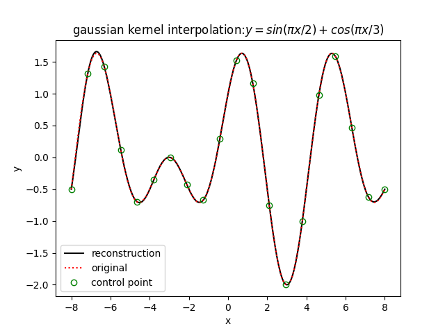
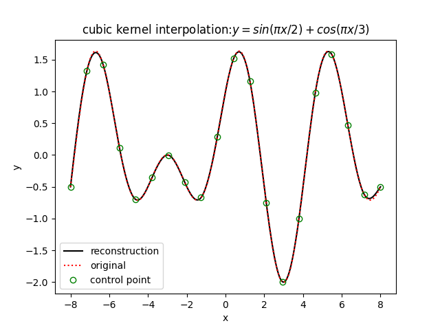
测试结果如下(一维插值):

总结
对于rbf插值中,一般控制点数量越多越密集,插值精度也就越高,但是随之而来的插值矩阵 $\Phi$ 增大,计算量增大,模型训练(权值系数计算)效率变低,正所谓“No Free Lunch”。其次,不同的基函数在同样的数据上插值的表现也有所差异,因此需要选择最优的基函数进行插值计算。
参考
[1] https://blog.csdn.net/xfijun/article/details/105670892
[2] https://zhuanlan.zhihu.com/p/339854179